Learn python for data analytics in one afternoon

Get started with data analytics in python. Learn from an experienced data scientist.

It’s Sunday afternoon. You start your new python job on Monday morning. During the interview, you managed to convince them that you know python. Now it’s time to actually learn a little bit of python - enough to survive your first week.

Aspiring data scientists might be laughing at the situation. Seasoned professionals know how common this scenario really is.

You might be thinking, “what’s so special about this python tutorial? There are bazillions of python tutorials on the internet.” It’s written by someone who has actually worked in the data analytics industry - who has a clue about what you might need to learn quickly. Competing articles might be written for resume building purposes. My resume is long enough without this article.

We will be using the “Bank Marketing” dataset from the UCI Machine Learning Repository. Grab the dataset now. It’s best if you follow along on your machine.

What’s Not Covered

I assume that you’re proficient in at least one other programming language. This tutorial does not cover variables, data types, flow control, functions, classes and anything that you will find in a generic “intro to programming” tutorial. You are here to learn what you need for data analysis - it’s not a first year computer science course.

I assume that you have already chosen how you will run your python code. Whether you will be copy-pasting into the REPL, using a notebook, executing your code from a file or something else. You have discovered that python uses indentation instead of brackets. Copy pasting indented code into the REPL does not always work too well - but I assume that you have it under control.

Sometimes installing a python package is easy as typing pip install mypackage in terminal. Other times it’s like solving a puzzle. I assume that you can debug python package installation on your specific machine when things go wrong. Or that you are using a python distribution that “just works” such as Anaconda.

For example, if you are using Ubuntu 18.04, then you will have to run the following command before setting up your virtual environment and installing python packages. sudo apt install python3-matplotlib

A Note on Notebooks

Notebooks solve the problem of pasting python code into terminal. Analytics requires trial and error. This means interactively iterating on your code. Each iteration may take you down that was not pre-planned. It is not feasible to implement pre-planned functionality, push it, close the ticket and then think about improvements - that’s engineering. Analytics is not engineering. Hence we need to run our code interactively. Either in a notebook or in a REPL (Interactive Mode). I prefer a REPL, your employer may force you to use a notebook.

The first notebook was the iPython/Jupyter notebook. To productionise code that is in a Jupyter notebook, you should take it out of the notebook and make it run in .py files. On the other hand, I once saw a software vendor present their own type of notebook. It appeared that you could productionise their proprietary notebooks on their proprietary system. As a rule of thumb, assume that code in notebooks will need to be heavily modified before deployment into production.

Virtual Environments

We work in virtual environments when using python for analytics. With virtual environments, we versions of packages that we use in our project from versions installed with the “system” python. It may not be a concern to you if you are using your company’s in-browser Jupyterlab instance.

Setting up a virtual environment

Here’s how we set up a virtual environment in terminal. We’ll start by creating a creating a new folder for our project.

~$ mkdir my_tutorial
~$ cd my_tutorial/

If you are using Ubuntu 18.04 or earlier or macOS 12.3.1 Monterey or earlier, you will have Python 2 and Python 3 running side-by-side. We will be using Python 3.

Python 3 introduced breaking syntax changes. Migrating code from 2.7 to 3 required some work. On older systems we call Python 2.7 with python and Python 3.x with python3. However, once we have activated our Python 3 virtual environment, python maps to Python 3.x.

Here’s how you set up a Python 3 virtual environment on those older systems.

~/my_tutorial$ python3 -m venv my_virtual_env

Newer operating systems will only have Python 3. Below is how you set up a virtual environment on those newer systems. The difference is only one character.

~/my_tutorial$ python -m venv my_virtual_env

In the example above, we have created a folder for this tutorial and then created the virtual environment that we will be using.

We will now activate our virtual environment and start the python interpreter in terminal.

~/my_tutorial$ source my_virtual_env/bin/activate
(my_virtual_env) ~/my_tutorial$ python

Note the python version. The example below is from Ubuntu 18.04.

Python 3.6.9 (default, Mar 15 2022, 13:55:28) 
[GCC 8.4.0] on linux
Type "help", "copyright", "credits" or "license" for more information.
>>> 

Now type quit() and press enter in the interpreter to exit.

We deactivate the our virtual environment with the deactivate command.

(my_virtual_env) ~/my_tutorial$ deactivate
~/my_tutorial$ python

Note the python version when calling python outside of the virtual environment. The example below is from Ubuntu 18.04.

Python 2.7.17 (default, Mar 18 2022, 13:21:42) 
[GCC 7.5.0] on linux2
Type "help", "copyright", "credits" or "license" for more information.
>>> 

At one point, there was a herd of programmers who refused to move to Python 3. Even after most libraries had been ported to Python 3. Python programming tutorials had a “which python should I learn” section - when it was clear that Python 2 will soon be old junk. Eventually the herd recognised that Python 3 is the correct version for the present day - but they could have done so years earlier.

Installing Python Packages

Now we’ll install the packages that we’ll be using. The example below uses pip. However, you might be using something else such as conda. They might be pre-installed if you are using your company’s in-browser Jupyterlab instance.

~/my_tutorial$ source my_virtual_env/bin/activate
(my_virtual_env) ~/my_tutorial$ pip install pandas matplotlib pyyaml

Reading Data

Download Our Tutorial Dataset

Download bank.zip from the UCI Machine Learning Repository. Extract bank-full.csv into your project folder. That’s the only file that we will use in this quick tutorial.

Create Config Files

Production code has config files. Learn to use them now. Don’t wait for your manager to tell you this. Config files are usually either YAML or JSON. I’ll teach you to work with both. Open a text editor and create the following files. Make sure that you replace “path/to/folder/with/bank-full/dot/csv” with an appropriate path.

file_io_config.yaml

data_folder: path/to/folder/with/bank-full/dot/csv
data_file: bank-full.csv

analytics_config.json

{
    "show_num_rows": 17,
    "histogram_config":
        {
            "color": "#33AA11",
            "title": "Histogram of Account Balances",
            "x_label": "Balance ($)",
            "y_label": "Number of Accounts",
            "num_bins": 120
        }
    
}

Reading Config Files

Here’s an example of loading the config files. Create a blank .py file or notebook and follow along.

#This is a code comment
#Example of loading JSON and YAML config files
import json
import yaml

#1. Read the YAML config
with open("file_io_config.yaml", 'r') as the_yaml_config:
    file_io_config = yaml.safe_load(the_yaml_config)

#2. Read the JSON config
with open("analytics_config.yaml", 'r') as the_json_config:
    analytics_config = json.load(the_json_config)

The config files have been read in as dictionary objects. You can access individual config items by specifying their names. For example, file_io_config['datafile'].

>>> file_io_config['datafile']
'bank-full.csv'

>>> analytics_config['show_num_rows']
17

Reading Data Files

You might have heard of the famous pandas library. It’s a python implementation of DataFrames. Even if your employer prefers some other DataFrame library, it will probably be “pandas-like”.

import pandas as pd

#Read the file path from the config
#Use + to concatenate strings
path_to_file = file_io_config['data_folder'] + '/' + file_io_config['data_file']


#Read the data
bank_customers = pd.read_csv(path_to_file, header=0, sep=";")

You can view the your freshly loaded dataset with bank_customers.head()

header=0 means that the header labels are in the top (or “0th”) row. sep=";" means that the file uses the semicolon character to separate the columns - not a comma.

Subsetting Data

Follow along with the examples below.

Basic Attributes

#Column names
bank_customers.columns

#Number of rows and columns
bank_customers.shape

Basic Access

#Show the top five rows
bank_customers.head()

#Show the top n rows - configurable
bank_customers.head(analytics_config['show_num_rows'])

#Get rows 3 - 7
bank_customers.loc[3:7,]

#Get rows 3 - 7, specific columns
bank_customers.loc[3:5,['job','marital']]

#Get the duration column
bank_customers['duration']

#Get each customer's job, marital status and education
bank_customers[['job','marital','education']]

#Another way to access individual columns. 
# Getting the y column in this case.
bank_customers.y

Filtering

#Get all of the customers with more than $1000
bank_customers[bank_customers.balance > 1000]

#Get all of the customers with more than $1000 AND who are single
bank_customers[(bank_customers.balance > 1000) & (bank_customers.marital == 'single')]

Cleaning Up The Data

We’ve loaded the data but it’s not quite ready to work with. We need to replace “unknown” strings with NaNs. String columns need to be cast as categorical. Ordered categories need to be modified in such a way that machine learning algos will know that they are ordered. “Yes”/”No” variables need to become binary 1/0s.

We will use numpy.NaN from the numpy library to represent missing values. Machine learning libraries should be able to understand that this is how we represent missing values. Follow along with the examples below.

import numpy as np

#Convert the y column to binary
bank_customers.y = np.where(bank_customers['y'] == "yes",1,0)

#The pdays column denotes missing values with 999.
# Replace 999 with NaN
bank_customers.pdays = np.where(bank_customers['pdays'] == 999,np.NaN,bank_customers.pdays)

#Replace 'unknown' with NaN
bank_customers.replace('unknown',np.NaN,inplace=True)

#Cast categories as categorical data types
bank_customers.loc[:,['job','marital', 'poutcome', 'contact']] = bank_customers.loc[:,['job','marital', 'poutcome', 'contact']].astype('category')

Here’s how check if any columns in the DataFrame have NaNs. They should be there because we put them there.

bank_customers.isna().any()

Here’s a function to convert “yes”/”no” variables to 1/0 variables. It’s just one line of code. It’s saves us from replacing “the_series” with variable names several times.

def convertYesNoToBinary(the_series):
    """
    Converts a Yes/No series to a 1/0 series
    """
    return np.where(the_series == 'yes',1,np.where(the_series == 'no',0,np.NaN))

Here’s how it’s used.

bank_customers.default = convertYesNoToBinary(bank_customers.default)

bank_customers.housing = convertYesNoToBinary(bank_customers.housing)

bank_customers.loan = convertYesNoToBinary(bank_customers.loan)

When we have an ordered categorical variable, we want to encode the ordering. For example, we will turn [‘primary’, ‘secondary’, ‘tertiary’] into [0,1,2].

bank_customers.education = np.where(bank_customers.education == 'tertiary',2,np.where(bank_customers.education == 'secondary',1,np.where(bank_customers.education == 'primary',0,np.NaN)))

Summary Statistics

We can get the summary statistics for each column of the dataframe with bank_customers.describe(). However, we might only get a subset of columns printed to the screen. You can switch off the column print limit with pd.set_option("display.max_columns", None).

You can reset the column display limit to a non-negative integer as well.

You can also describe subsets of the DataFrame.

#View summary stats of customer account balances
bank_customers['balance'].describe()

#View summary stats of balances of customers with a tertiary education

bank_customers[bank_customers.education == 2]['balance'].describe()

Dropping Columns

bank_customers = bank_customers.drop('duration',axis=1)

axis=1 tells the drop() function that it should look for a column named ‘duration’. The default behaviour is to look for a row name ‘duration’.

Creating X matrices and Y vectors

X = bank_customers.drop('y',axis=1)
y = bank_customers.y

Charts, in matlotlib.

Using a Matplotlib backend

Matplotlib is the charting library for python. Sure there are other libraries, but a lot of them depend on matplotlib. Matplotlib uses backends to draw the charts. Some backends are “interactive” - the kind that make a chart pop up in a new window. Other backends will write to a file. The commands below can used the view the list of supported backends.

matplotlib.rcsetup.interactive_bk
matplotlib.rcsetup.non_interactive_bk
matplotlib.rcsetup.all_backends

If you are using a Jupyter notebook, then you will need to set the inline backend.

%matplotlib inline

If you are using python in the terminal on Ubuntu 18.04, then the following should work.

import matplotlib
matplotlib.use('TkAgg')

Plotting a histogram of account balances

We have stored our chart parameters in our analytics_config.json file.

import matplotlib.pyplot as plt

h_conf = analytics_config['histogram_config']

the_histogram = plt.hist(bank_customers.balance, 
    h_conf['num_bins'], 
    color=h_conf['color'])

plt.xlabel(h_conf['x_label'])

plt.ylabel(h_conf['y_label'])

plt.title(h_conf['title'])

plt.show()

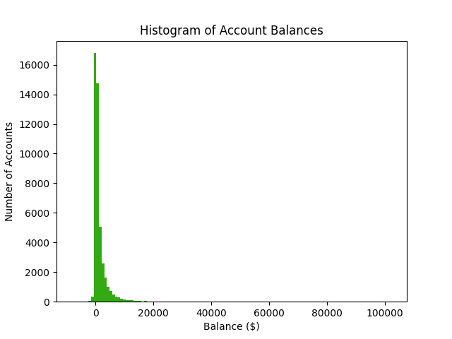
Why does my histogram look like that?

Wealth and bank account balances follow a Pareto distribution. Hence most bank accounts have a balance that is close to zero. There are a few values in the far right tail, which make the rest of the histogram look really zoomed out. Read my article on fat tailed distributions here.

Here’s how we could further investigate the distribution of account balances in python. The np.arrange() function is used to create an list of quantiles.

#Get the 10 largest account balances
bank_customers.balance.nlargest(10)

#Summary stats. Note how that 3rd Quartile(75%) is not all that high.
bank_customers.balance.describe()

#Get the median
bank_customers.balance.median()

#Calculate the quantiles at 5% increments
ntiles = np.arange(.05,1,.05)
bank_customers.balance.quantile(ntiles)

#Calculate the quantiles from 99% to 100% at 0.1% increments
ntiles = np.arange(.99,1,.001)
bank_customers.balance.quantile(ntiles)

Remember to subscribe to keep learning.

Good Luck!

I hope to have picked up enough python to get started on Monday morning. When you need to look something up, you now know what to look for - and what you are actually copy-pasting from Stack Overflow. Remember to use config files for any code that is going into production in the future.

We have touched on fat tailed distributions when we explored the customer account balances. Read my article on fat tailed distributions here. Make sure that you receive all future updates - don’t miss out. Subscribe now to stay up to date and keep learning.

This article might be the first time that you have seen this newsletter. You might be wondering what the broader newsletter is about. Follow this link to read how you can get an edge in your career.